
Weekly Forecasts 22/2026
The mystery of statistical forecasting and an update to the U.S. GDP forecasts (Free)

Contents:
Restructuring the forecasting model of U.S. real gross domestic product (GDP).
Updated forecasts for U.S. real GDP.
A preliminary look at the forecasting of the GDP of the Eurozone.
This week, we’ll dive relatively deep into the realm of statistical analysis. What we will present to you is, first, an update and an extension to our GDP forecasting model. We retested the assumptions behind our model and adjusted it accordingly. This was done to check whether data updates and revisions had changed something, and they had.
It now looks like the “correct” cointegration rank of our system of three equations (variables) would be one, instead of two we used previously. While this may sound like statistical jargon, such assumptions do affect the statistical estimator and hence the forecasts it produces. Still, the “corrected” model finds that the U.S. economy would enter something of a mini-collapse in this quarter.
Because the high-frequency data we have on the U.S. economy does not support such a scenario, we consider it relatively unlikely. However, the model’s primary objective has consistently been to predict turning points, not to accurately forecast the growth rate of the U.S. economy (we have not yet even tried to calibrate it to be accurate). Hence, while the collapse is unlikely to occur now, we wait with interest to see whether this quarter will be the turning point for the U.S. economy.
Lastly, we take a preliminary look into the forecasting of the real GDP of the Eurozone. The construction of the model is met with several challenges, which we start to map here. Thus, we do not provide any forecasts for the development of the economy of the Eurozone yet.
I also like to remind you of our summer campaign, which offers our annual subscription with 30% off.
Tuomas
Restructuring the forecasting model for U.S. GDP
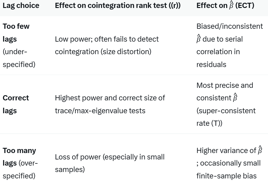
In this section, we detail how we used the autocorrelation functions and the error correction framework to check and partly remodel our forecasting model. In practice, we sought the smallest number of lags that was able to control for autocorrelation and partial autocorrelation but which also produced an appropriate error correction presentation of the underlying long-run dynamic (cointegration). Per Grok Expert:
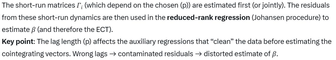
This means that if the auxiliary regressions (you can refer to these as “preparatory regressions”) used to assess or uncover the nature of the underlying cointegration relationship are biased, then the estimated coefficient for the cointegration vector (beta) and hence the error correction presentation will also be biased. From Grok Expert:
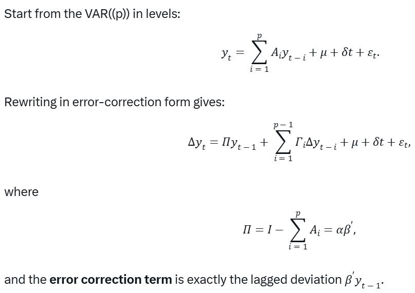
This is the very basic presentation of the ECT. What the lag structure of the auxiliary regressions affects is the estimated presentation of the last term (vector) beta. In other words, if this estimate is biased, so will the error correction term. See the full summary from the footnote.1
Testing for the correct lag structure in the VECM is not easy or simple. We applied a two-staged method. We observed both the autocorrelation functions and the error correction term (EC) term.
To remind you, error correction terms are such that, if cointegration between two (or more) I(1) nonstationary variables exists, they present the path of the series returning to the equilibrium defined by the (stationary) cointegration relationship. If an EC term, for example, exhibits an upward or a downward trend, or “wanders,” it is either not well defined (incorrectly estimated, see above) or it captures a deterministic trend or stochastic trend process. This feature can also be used to assess whether the lag structure of the (auxiliary) regressions is correct and to assess the rank of cointegration in the system.2
We started by re-running the unit root and cointegration tests for the updated values of the three variables: the U.S. (seasonally adjusted) Real Gross Domestic Product (RGDP), Gross Private Domestic Investments (GPDI), and Loans and Leases in bank credit (LL) from Q1 1947 until Q1 2026. They brought upon one change. The Johansen Trace Test now indicated that there would exist one stationary cointegration vector between the three variables instead of the two it found the last time.
To test this change further, we took natural logarithms from all three series to smoothen their distribution and linearize the series.3 The extreme values (peaks and drops) make it more difficult to find a correct lag structure, as the extreme values usually carry a long-time effect in the series, which can require a (considerably) longer lag structure to control for what would be needed without them. “Over-lagging” leads the model to lose the power to correctly identify statistical restrictions. With the Johansen Trace Test, this implies that the test can, for example, over-identify the number of cointegration vectors.
The Johansen Trace Test, run with the (natural) logarithmic values of RGDP, GPDI, and LL, indicated that there would exist one (stationary) cointegration vector between the three variables. In other words, the test implied that three variables would share the same stochastic trend. Thus, we took the cointegration rank of one as the basis of the VECM.
Next we ran several estimations with the three-variable VECM system, assuming different lag structures. We started with the smallest amount of lags suggested by BIC (Bayesian Information Criterion), which were unable to account for the autocorrelation. We started to grow the number of lags and, at the same time, we observed how the error correction term behaved. If it, e.g., exhibited a trend, we changed the lag structure.4 Figure 1 presents the error correction term of the VECM model we ended up using.5
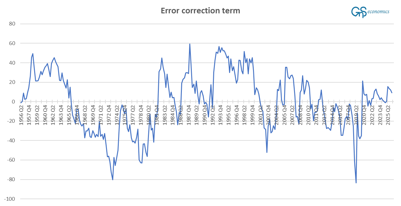
The error correction term of our model behaves as it should, mostly. It fluctuates around zero without any clear time structure or a trend, while it “wonders” a bit. Unit root tests find it to be stationary, but only barely (the ADF test rejects the unit root in the series at the 5% but not at the 1% level). This warrants further study, later.
The exercise presented in this first section should make our forecasting model more reliable, statistically speaking. The extensive retesting indicates that our model is (more) sound or, more precisely, that the underlying assumptions seem to be correct. This naturally does not guarantee that the model is good, i.e., that the forecasts it produces are accurate, which is only something time can tell.
Let’s now turn to the forecasts our updated model provided.
Forecasts for U.S. GDP
In practice, the only things that truly change in our model are the assumed rank of cointegration in our system of three equations and the lag structure. These changes do not change the implications of our forecast much, as you will notice below. Note that we do not provide scenario forecasts this time because we want to see how our updated baseline model performs and what comes from the Middle East.
Let’s start by checking how the Q4 forecasts of our baseline model performed. Figure 2 presents our forecasts from February 23.
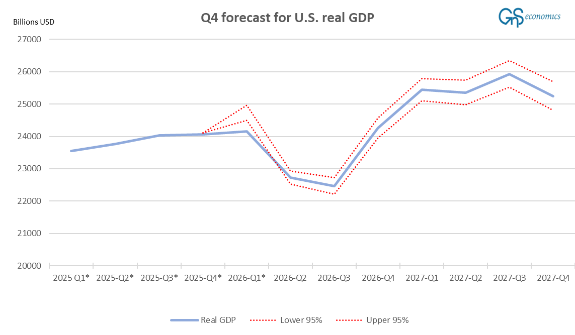
Like you notice, the realized value of U.S. real GDP went straight through the lower (95%) confidence interval of our forecast. This simply means that our model failed to forecast the short-term development of the U.S. GDP. This has been the tendency of our model since Q3. That is, the model tends to exaggerate the change in the U.S. real GDP, but like we noted above accuracy is something we have not aimed with it, yet. We have to emphasize, though, that our oil crisis and financial crisis scenario forecasts got close to the actualized GDP print (the second estimate for Q1 2026 GDP was $24152 billion). Keeping this in mind, what does the model see coming next?
Figure 3 depicts our updated forecasts using the model constructed above.
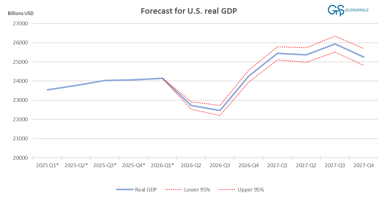
The model still sees the Q2-Q3 slump in U.S. GDP followed by a strong recovery. What makes this result so perplexing is that, while the model has gotten the magnitudes of U.S. real GDP growth mostly wrong in the past, it did correctly foresee the acceleration of the U.S. economy during Q2 and Q3. It has also consistently forecasted a slump for the U.S. economy for Q2 and Q3 this year.
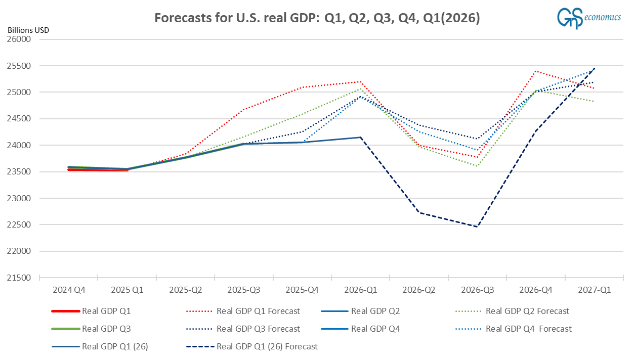
This consistency is what perplexes us. Oftentimes one sees an econometric forecasting model to anticipate a down- or upturn but postpones its onset with new or revised data. The prediction of our model of the Q2-Q3 slump of the U.S. economy has not changed through several revisions, some of which changed the GDP figures notably, and through four new data points (Q2, Q3, Q4, and Q1).
However, while the U.S. consumer is hurting, for example, the Aruoba-Diebold-Scotti Business Conditions Index, which we have been using as a basis for our nowcasts of U.S. GDP growth, does not show such a collapse. It is thus likely that our model is exaggerating the magnitude of the downturn. Hence, the real question becomes whether it has correctly identified the downturn starting in this quarter? Based on its consistency, we are keen to think so, but the only way to find out is to wait.
Forecasting the Eurozone real GDP
Let’s now take a quick first look at forecasting the real gross domestic product of the Eurozone. The macroeconomic variables available for the Eurozone differ a bit from those of the U.S. While the real GDP is essentially calculated the same way everywhere, Eurostat does not currently provide gross private domestic investments. Hence, we rely on gross fixed capital formation, which is a broader measure including, e.g., military spending.
The gross fixed capital formation, or Investment series is “messy,” and there are several options for how to calculate it: unseasonal, seasonal, calendar, etc. We selected a series that is both seasonally and “calendar” adjusted. The latter “smoothens” the effect of national holidays, etc., which are automatically removed from, e.g., the FRED database of the Fed St. Louis. This is the first time we heard about such, and we consider it problematic in the sense that it makes the series more artificial by essentially guessing (statistically) what the effect of these holidays is on the gross fixed capital formation.6 Figure 5 presents the time series of the Eurozone’s real gross domestic product and gross fixed capital formation.
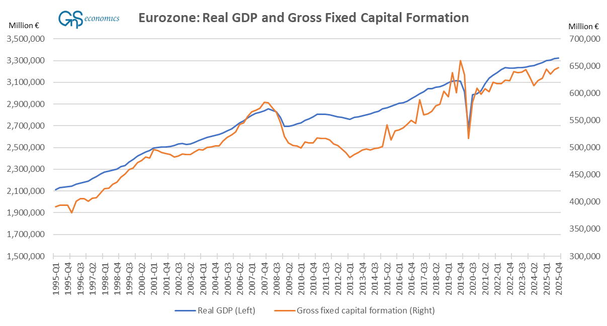
The similarity with the relationship between the U.S. (seasonally adjusted) Real Gross Domestic Product and Gross Private Domestic Investments and Figure 5 is obvious, but the relationship of the U.S. variables looks much tighter. The likely reason for this is that private investments tend to be more productive than government (federal) investments, which are included in the gross fixed capital formation series, and thus contribute more to the GDP (hence the co-movement).
This leads us to the first problem in our forecasting setup for the Eurozone’s GDP. While the ADF (Augmented Dickey-Fuller) test finds that the two variables are unit root processes with a drift, the Johansen Trace Cointegration test does find them to be cointegrated. What this implies is that the two series would be driven by different stochastic trend processes.
The above indicates that we cannot estimate the two variables as a system, because adding two non-cointegrated I(1) integrated processes into the same model leads to a spurious regression problem (more on this sometime later). We could go around this by first-differencing the variables, which removes the stochastic trend process. This would counterproductive for our aim, because it would remove the long-run driving force of the series, i.e., the stochastic trend.
However, the most important thing for you to understand about statistical analysis is that essentially nothing can be proved to be “right or wrong”.7 Hence, more research is needed to know whether the above results hold true. As this report is already several pages long, we’ll leave this for the future.
Disclaimer:
The information contained herein is current as of the date of this entry. The information presented here is considered reliable, but its accuracy is not guaranteed. Changes may occur in the circumstances after the date of this entry, and the information contained in this post may not hold true in the future.
No information contained in this entry should be construed as investment advice nor advice on the safety of banks. GnS Economics, Tuomas Malinen, or other authors cannot be held responsible for errors or omissions in the data and information presented. Readers should always consult their own personal financial or investment advisor before making any investment decision or decision on banks they hold their money in. Readers using this post do so solely at their own risk.
Readers must assess the risks and legal, tax, business, financial, or other consequences of their actions. GnS Economics, Tuomas Malinen or other authors cannot be held i) responsible for any decision taken, act, or omission or ii) liable for damages caused by such measures.
Summarization by Grok Expert:
The error correction terms can be used to assess the rank of cointegration in a system of equations. In our system of three equations (variables), we can assume a cointegration rank of two in the VECM, estimate the model, and draw out the EC terms. If the series appears like in Figure 1, we can assume that the number of stationary cointegration vectors in our system is two (rank=2).
If, however, one of the EC terms exhibits clear trending or “wondering” behavior, it implies that the error correction term is including something else than the deviation of the variables from their long-run (stationary) cointegration relationship. This happened to us when we estimated our system of three equations with VECM, assuming a cointegration rank of two. This further emphasizes that the actual cointegration rank of our system is likely one.
Taking logarithms stabilizes a time series because it smoothens the distribution of the series by diminishing extreme values (which may be a result of, e.g., measurement error) and linearizing the series.
Note that a deterministic time trend was included in the VECM model.
The VECM model included a constant, a deterministic time trend, and 35 lags of endogenous variables (U.S. real gross domestic product, gross private domestic investments, and loans and leases in bank credit), assuming a cointegration rank of one. The lag structure was able to remove most of the autocorrelation and partial autocorrelation (up to 42 lags) from the residuals. Some autocorrelation in the squared residuals and heteroscedasticity remained.
Furthermore, the composition of the Eurozone has changed (grown) since its establishment on 1 January 1999, when it initially included 11 member states. Currently it holds 21 member states. This means that over the course of the past 17+ years, the statistical composition of the monetary union has changed, and data from new member countries were added to the statistical metrics of the Eurozone retroactively. Although technically feasible, such an addition can lead to errors and other statistical issues.
The econometrics teacher of Tuomas at the Master’s level, Professor Markku Rahiala, emphasized this constantly.