
Weekly Forecasts 11/2026
U.S. inflation in an oil shock and supply chain collapse scenarios

Contents:
The U.S. inflation picture in February.
Forecasts for U.S. inflation assuming no oil shock scenario.
Forecasts for U.S. inflation under an oil shock and supply chain collapse.
The war in the Middle East rages on. Patricia published an excellent analysis on the worrying trajectory of the conflict yesterday. If you have not, I urge you to check it out. It is free to read.
This week, we’ll continue to assess the economic effects of the war, concentrating on the U.S. Most of the effects arise from the closure of the Strait of Hormuz. Writing about it now is even a bit surreal considering that I warned of the (dire) economic effects of the closure already in October of 2023. The interesting recent twist in it is that “Petroyuan” can break the closure relatively soon, as it looks like Iran allows passage to ships that stay away from the conflict and buy their oil with Renminbi. This, i.e., the beginning of an end of the petrodollar, is essentially what we speculated would occur last week.
Another positive development is that rumors of serious infighting within the Trump administration have started to appear. According to them, Vice President James David Vance would be strongly opposing the continuation (and deepening) of the war. My current thinking is that we could see an end to the conflict by the end of April. Let’s see (I’ll detail them later).
Regardless, an economic shock is already on its way and the only question is, how bad will it get? Reports of high prices at the pump in the U.S. and even fuel shortages emerging in Asia have started to emerge. The path of inflation is dictated by heavy uncertainty.
We will provide a path through the uncertainty with the help of two scenario forecasts detailing the possible paths of U.S. inflation for the next 12 months. We start with standard forecasts, which include no specific information on the approaching shock. These forecasts act only as a benchmark, as the shock is already emerging, and it will get worse, even if the war ends tomorrow. The more serious scenarios encompass an oil (energy) shock and disruption of global supply chains. Naturally, the latter of these paints a very detrimental path for the U.S. economy going forward. Our assessment is that, if the war continues, we will start to move into the supply-chain collapse scenario after next week.
Tuomas
The state of U.S. inflation
Let’s first check how our inflation forecasts from the past month fared. In February, the Consumer Price Index (all items, all urban consumers, U.S. city average, seasonally adjusted), or CPI, rose by 2.4% annualized, 0.3% month-over-month (MoM). The core inflation rose by 2.5% annualized and 0.2% MoM. The “super-core,” i.e., services less energy costs, rose by 2.9% annualized, 0.3% MoM.
Our forecasts, from 17 February, indicated that the CPI would increase, month-over-month, by 0.3%, the core inflation by 0.4%, and the super-core by 0.3% in February. In other words, our forecasts accurately predicted the rate of change of CPI and supercore inflation, but they failed to foresee the deceleration of core inflation. Every realized figure was within the 95% confidence intervals, though. Figure 1 presents our February forecasts and the realized value for the MoM change in core inflation with 95% confidence intervals.
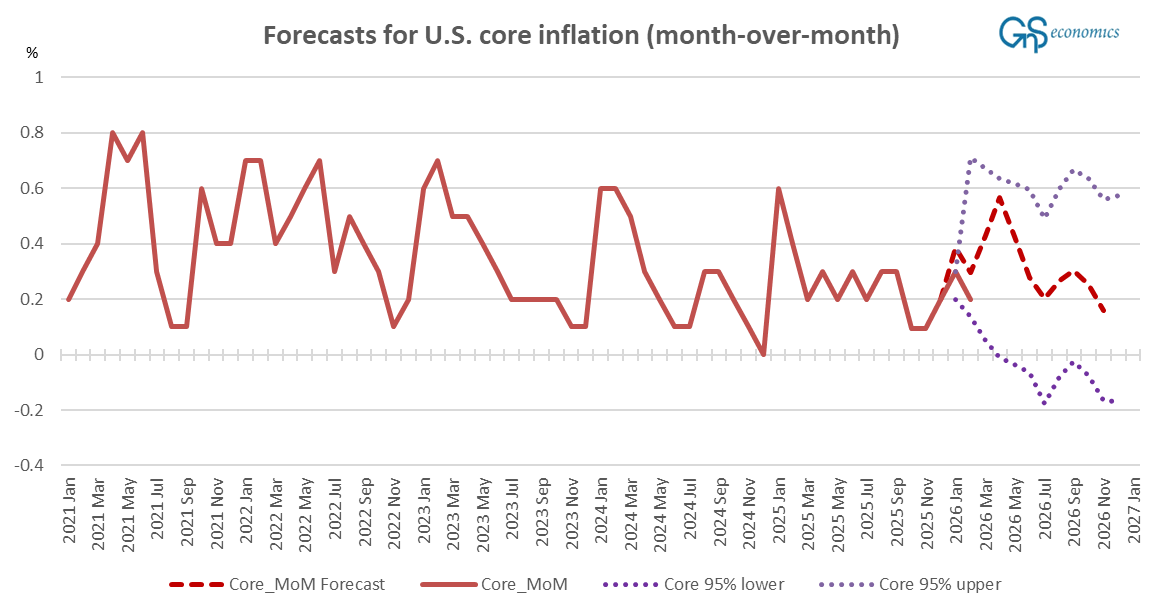
Given the accuracy of our forecasts for the CPI and super-core inflation, it’s plausible that the deviation from the core is merely a random statistical event. What this means to say is that no forecast can be assumed to be 100% accurate, but there’s a stochastic variation in the forecasts based on the assumption of the underlying probability distribution. All statistical forecasts are of the form: estimate +/- the margin of error, where the “estimate“ or “point estimate” is the term for the actual forecasted value and the margin of error is the assessment of the model on the fluctuation of the forecast based on the underlying distribution and the predetermined threshold. In economic sciences, 95% is generally used as a threshold for “statistically significant” observation (and forecast), while, for example, in physics, much tighter thresholds, like 99.999%, are oftentimes used. This difference arises from the fact that stochasticity (randomness of observations) in measured physical phenomena is generally much smaller than in economics. Just think of it as a difference between the actions of men vs. laws of physics. Thus, at this point we do not make any major changes to our forecasting model, because the miss in our core inflation forecast can be just random statistical variation.
But where is U.S. inflation heading? Figure 2 presents the recent monthly changes in the three key inflation metrics.
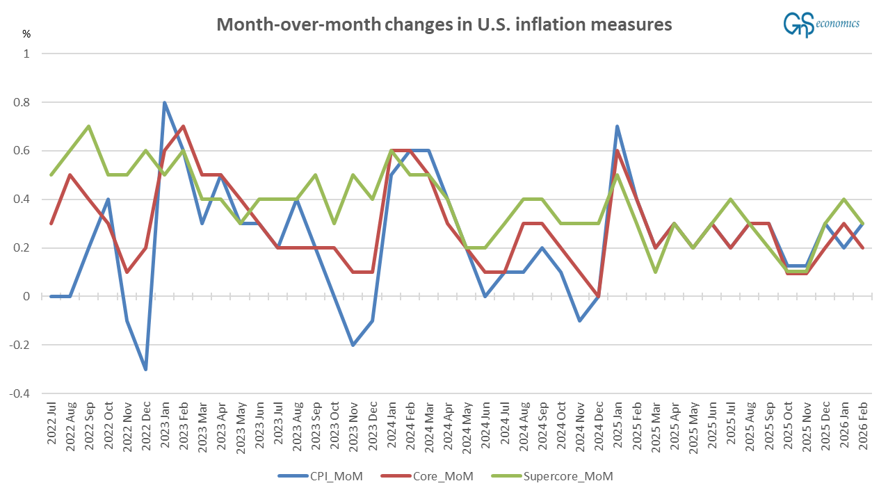
What we have seen, since the shock the onset of the war in Ukraine created in 2022 started to ease about a year ago, is a stabilization after a relatively long period of heavy fluctuation. The problem is that this is about to change abruptly due to the shock arriving from the Middle East. We do not know its length and depth, though, because it is determined by political decisions of leaders concerning the Gulf region and their impacts on global markets. We naturally specialize in addressing such uncertainty through scenario forecasting. Let’s first provide the “baseline” by updating our standard inflation forecasts.
Forecasts for U.S. inflation in the no-oil-shock scenario
We extend the forecasting model from February to also include the (monthly) supercore inflation, following the update (and correction) made by Tuomas. This modification diminished the mean squared errors of the model somewhat, which implies that the super-core is providing information that is helpful in modeling and forecasting the system of three variables: CPI, core inflation, and supercore inflation. Otherwise, we use the same setup as in February.
We approximate the monthly U.S. CPI, core inflation, and super-core inflation series with a stochastic trend process. That is, we assume, based on the results of the Augmented Dickey-Fuller (ADF) test indicating that the series contain unit roots, that the series are driven by stochastic trends. The Johansen Trace Test with updated data indicates that two stationary cointegration vectors would exist between the three variables (using a 5% level of statistical significance). We then applied the Vector Error Correction (VECM) to estimate the model and forecast the path of the three inflation measures for the next 12 months.1 Figure 3 presents the forecasts it yielded.2
