


We analyze the time series properties of the price of Bitcoin.
Is supply liquidity the long-term driver in the price of Bitcoin?
What are the short-run effects of liquidity injections into the price of Bitcoin?
First (preliminary) forecasts for the price of Bitcoin.
This week, we take up on forecasting the price of Bitcoin, an endeavor we have been planning for a long time. We will not even try to offer you a comprehensive view or reliable forecasts this week, but to present you the first pieces of (statistical) information on the drivers of the price of Bitcoin.
We have been speculating for some time, how do global and U.S. liquidity injections affect the price of Bitcoin. This is our starting point this week and the results are a mixed bag. At this point, we are unable to identify a clear long-run dependency relationship between liquidity injections and the price of Bitcoin, but this does not mean it does not exist. We just have to deepen our analysis in the future to find out.
In the short run, our results suggest that changes in liquidity do influence Bitcoin, but the effects are temporary and fade relatively quickly. Forecasts built on this framework suggests continued volatility rather than a smooth trend, showing that short-term dynamics are more relevant than long-term dependencies for now. These first steps give us a starting point.
Tuomas and Mate
The time series properties of the price of Bitcoin
The main issue in building a forecasting model for the price of Bitcoin is its exceptional history. For a very long time, the price was very low, hovering near zero for most of 2009 and 2010. Then, in 2012, the price started to rise rapidly, passing the $1000 mark on January 4, 2014. However, the price quickly fell back below the $1000 mark, and it did not reach it again before January 2, 2017. From then on, the price started its spectacular rise to the current level in the vicinity of $110k.1
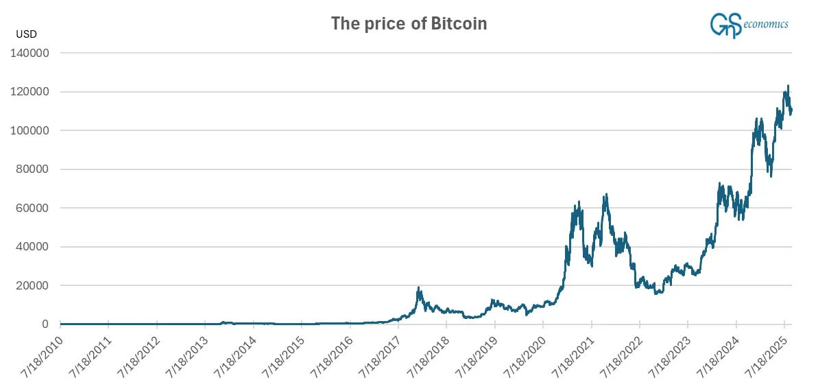
When it comes to time series analysis, Figure 1 raises one question above others. Does Bitcoin follow the same trend process throughout its history, or does it change, e.g., in 2017?
The above means that before 2017, the stochastic process behind Bitcoin may have been very different. Back then, it was bought mostly by “nerds” and loyal followers of Satoshi Nakamoto. In 2017 (or earlier), Bitcoin started to gather the interest of investors, shown by notable increases in its price. This implies that at that point, the process that drives its price changed, from “nerds” to investors, which also means that it became an actual financial asset. This implies that it would have been traded differently after 2017 (or even earlier).
Considering time series analysis, the above means that statistical properties of the series may have changed in 2017 (or earlier), implying a possible structural break. However, the massive appreciation in the price of Bitcoin masks any developments at the early stages of the series simply because of the sheer size of the increase in the price during the past few years. How one goes around this is through logarithms. Logarithmic conversion of a time series effectively presents the path of growth of the series. It thus eradicates the scale, or more precisely, changes it from a level to a path of change.2
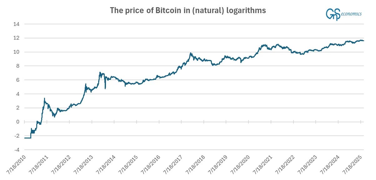
The logarithmic series of the price of Bitcoin presents an intriguing growth path. There’s nothing happening at the start (remember that taking natural logarithms from values between 0 and 1 will yield negative numbers). Then there’s a major growth spurt from around late 2010 until mid-2011. Moreover, from around mid-2014 on, while growing (and fluctuating) strongly, the price of Bitcoin has entered a growth path with a declining trend (shown by the slowly declining upward trend of the price series).
For time series analysis, Figure 2 implies that we should disregard all values prior to mid-2011, because the development of the price of Bitcoin is rather chaotic before that (first the price goes nowhere, then it faces a massive jump followed by a drop). While this all can be a part of a stochastic trend, the “chaos period” is almost surely driven by different underlying forces than what we see now. In 2011, there are also lengthy periods when the price does not change for days and days in a row. For these reasons, our statistical analysis covers the data from 1 January 2012 until now. This is how the autocorrelation and partial autocorrelation functions of the natural logarithm of the price of Bitcoin look.
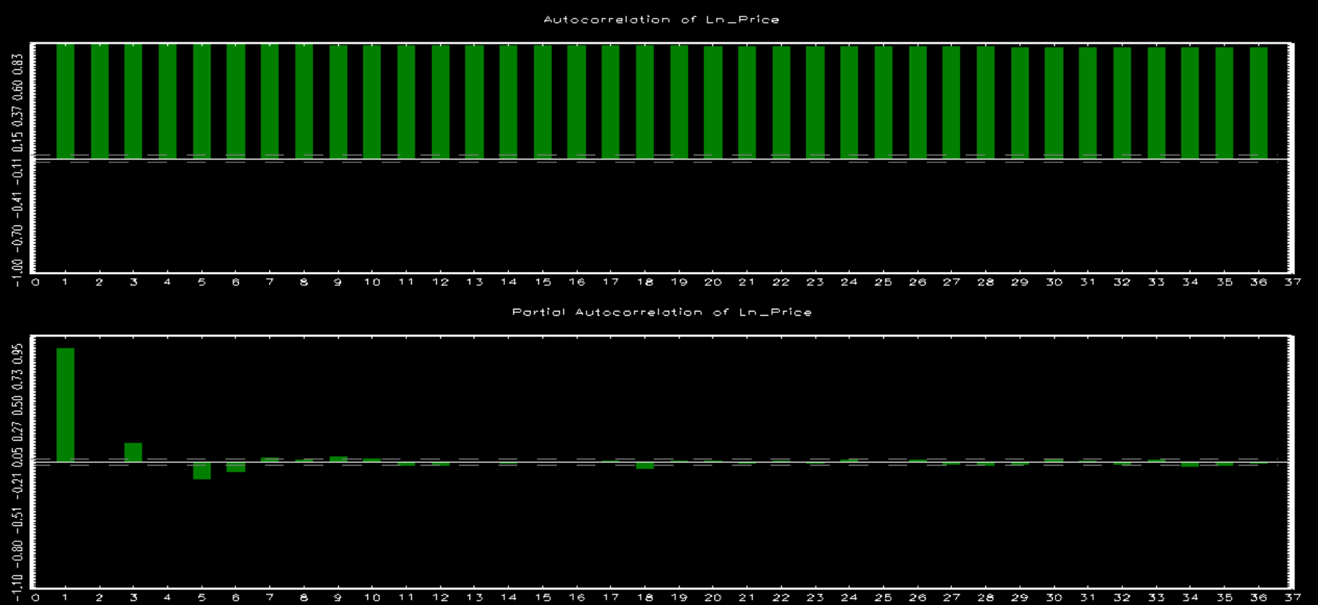
What we can see from the upper part of Figure 3 is that the time series of the price of Bitcoin has a very long, possibly “infinite,” memory. This suggests that the series would be an I(1) nonstationary process. Partial autocorrelation function, presenting the autocorrelation after removing correlation between shorter lags,3 shows a the first partial autocorrelation lag is very high (in the vicinity of 1). This implies that the process could be I(1) nonstationary. The ADF unit root test suggests that the price of Bitcoin would be a random walk with drift (a unit root process with a time trend).
To recap. A unit root (an I(1) nonstationary) process is effectively a statistical process which information set is unknown. This means to say that we do not know the different forces driving the series, which makes its time series wanders through time as driven by strong random shocks. In other words, the series looks like driven by a stochastic trend. This assumption fits perfectly with Bitcoin, because its price is affected not just by the decisions of a wide variety of investors but also by governments (like El Salvador) and authorities. Next we turn to analyzing some of these forces.
Analysis on the effect of liquidity flows on the price of Bitcoin
Like noted above, we have been speculating for long that liquidity flows could affect the prices of cryptocurrencies, especially that of Bitcoin. We’ve speculated that global liquidity injections, China’s liquidity injections, and the money supply (M2) of the U.S. could have an effect on the price of Bitcoin. Next, we put our hypothesis to the test.
