A mistake and forecasts

The liquidity train looks to roll on

Yesterday, I noted in the section introducing the impulse-response analysis that:

With this decomposition, ordering of the variables is important, because it is assumed that the first variable affects the other, but not vice versa. In this case, China comes before Total in our VAR model because there are grounds to assume that shocks to China’s money supply are dominant to the Total. As I write this, I realize that we have not been as careful with this assumption in the past as we should have been.

Today I have realized that we have forgotten to check this with many of our impulse-response analyses done during the past five months. While generally the ordering of the variables should have been correct, we have to redo and double-check a vast majority of our impulse-response analyses. I have to admit that at some point, we were too eager to proceed with the forecasting and forgot to check the theoretical foundations of our analyses. Therefore, this is mostly my 'bad'. This mistake should not have affected our forecasts (but we need to verify those too).

Today, I will provide simple time series forecasts for the global liquidity (money supply) flows. Yesterday, I realized that we also need to further develop the forecasts by adding more countries, but that is long process. Figure 1 shows how our forecasts performed.

Figure 1. Forecasted (with 95% confidence intervals) and actualized values of “Total” liquidity consisting of money supplies from China, the euro area, Japan, the U.K., and the U.S. Source: GnS Economics, PBoC, ECB, BoJ, BoE, Federal Reserve.

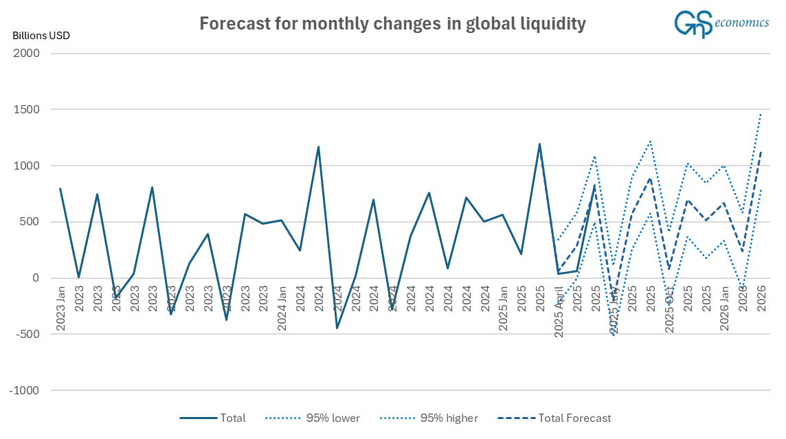
As you notice, our forecast indicated that the “Total” money supply would have grown a bit more rapidly from its stoppage in April. Our forecasts also indicated that we would not see a draining of liquidity in April, which materialized (the point forecast was an injection of $61 billion, while $40 billion was actualized). Our forecasted June liquidity injection ($793 billion) was also very close to the realized injection of $825 billion. This is how our updated forecasts look.